Quick start guide¶

This short guide shows the key steps in using BayesPy for variational Bayesian inference by applying BayesPy to a simple problem. The key steps in using BayesPy are the following:

Construct the model
Observe some of the variables by providing the data in a proper format
Run variational Bayesian inference
Examine the resulting posterior approximation

To demonstrate BayesPy, we’ll consider a very simple problem: we have a set of observations from a Gaussian distribution with unknown mean and variance, and we want to learn these parameters. In this case, we do not use any real-world data but generate some artificial data. The dataset consists of ten samples from a Gaussian distribution with mean 5 and standard deviation 10. This dataset can be generated with NumPy as follows:

>>> import numpy as np
>>> data = np.random.normal(5, 10, size=(10,))

Constructing the model¶

Now, given this data we would like to estimate the mean and the standard deviation as if we didn’t know their values. The model can be defined as follows:

$\begin{split} p(\mathbf{y}|\mu,\tau) &= \prod^{9}_{n=0} \mathcal{N}(y_n|\mu,\tau) \\ p(\mu) &= \mathcal{N}(\mu|0,10^{-6}) \\ p(\tau) &= \mathcal{G}(\tau|10^{-6},10^{-6}) \end{split}$

where $\mathcal{N}$ is the Gaussian distribution parameterized by its mean and precision (i.e., inverse variance), and $\mathcal{G}$ is the gamma distribution parameterized by its shape and rate parameters. Note that we have given quite uninformative priors for the variables $\mu$ and $\tau$ . This simple model can also be shown as a directed factor graph:

Figure made with TikZ

Directed factor graph of the example model.

This model can be constructed in BayesPy as follows:

>>> from bayespy.nodes import GaussianARD, Gamma
>>> mu = GaussianARD(0, 1e-6)
>>> tau = Gamma(1e-6, 1e-6)
>>> y = GaussianARD(mu, tau, plates=(10,))

This is quite self-explanatory given the model definitions above. We have used two types of nodes GaussianARD and Gamma to represent Gaussian and gamma distributions, respectively. There are much more distributions in bayespy.nodes so you can construct quite complex conjugate exponential family models. The node y uses keyword argument plates to define the plates $n=0,\ldots,9$ .

Performing inference¶

Now that we have created the model, we can provide our data by setting y as observed:

>>> y.observe(data)

Next we want to estimate the posterior distribution. In principle, we could use different inference engines (e.g., MCMC or EP) but currently only variational Bayesian (VB) engine is implemented. The engine is initialized by giving all the nodes of the model:

>>> from bayespy.inference import VB
>>> Q = VB(mu, tau, y)

The inference algorithm can be run as long as wanted (max. 20 iterations in this case):

>>> Q.update(repeat=20)
Iteration 1: loglike=-6.020956e+01 (... seconds)
Iteration 2: loglike=-5.820527e+01 (... seconds)
Iteration 3: loglike=-5.820290e+01 (... seconds)
Iteration 4: loglike=-5.820288e+01 (... seconds)
Converged at iteration 4.

Now the algorithm converged after four iterations, before the requested 20 iterations. VB approximates the true posterior $p(\mu,\tau|\mathbf{y})$ with a distribution which factorizes with respect to the nodes: $q(\mu)q(\tau)$ .

Examining posterior approximation¶

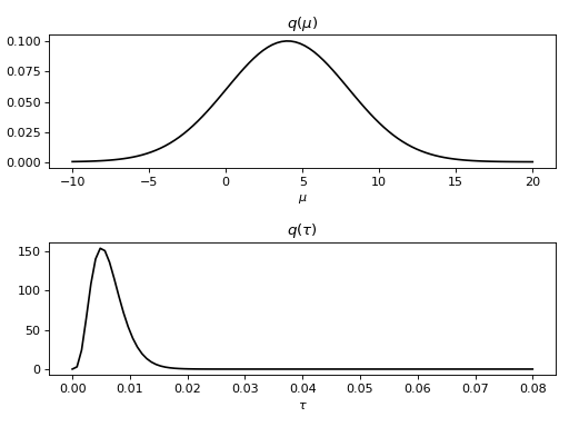
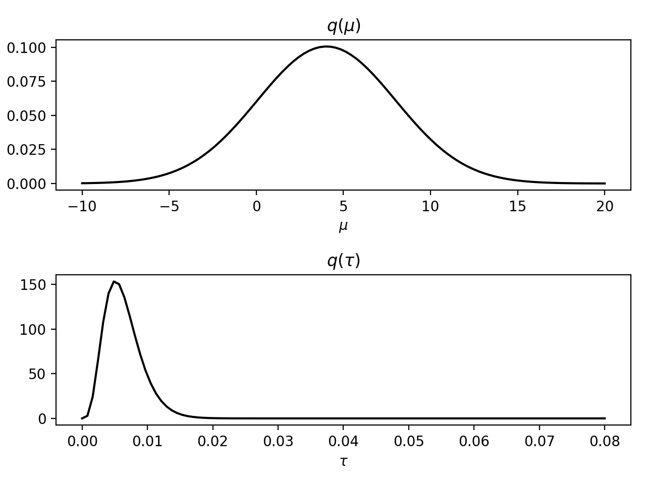
The resulting approximate posterior distributions $q(\mu)$ and $q(\tau)$ can be examined, for instance, by plotting the marginal probability density functions:

>>> import bayespy.plot as bpplt
>>> bpplt.pyplot.subplot(2, 1, 1)
<matplotlib.axes...AxesSubplot object at 0x...>
>>> bpplt.pdf(mu, np.linspace(-10, 20, num=100), color='k', name=r'\mu')
[<matplotlib.lines.Line2D object at 0x...>]
>>> bpplt.pyplot.subplot(2, 1, 2)
<matplotlib.axes...AxesSubplot object at 0x...>
>>> bpplt.pdf(tau, np.linspace(1e-6, 0.08, num=100), color='k', name=r'\tau')
[<matplotlib.lines.Line2D object at 0x...>]
>>> bpplt.pyplot.tight_layout()
>>> bpplt.pyplot.show()

(Source code, png, hires.png, pdf)

This example was a very simple introduction to using BayesPy. The model can be much more complex and each phase contains more options to give the user more control over the inference. The following sections give more details about the phases.