Hidden Markov model

In this example, we will demonstrate the use of hidden Markov model in the case of known and unknown parameters. We will also use two different emission distributions to demonstrate the flexibility of the model construction.

Known parameters

This example follows the one presented in Wikipedia.

Model

Each day, the state of the weather is either ‘rainy’ or ‘sunny’. The weather follows a first-order discrete Markov process. It has the following initial state probabilities

>>> a0 = [0.6, 0.4] # p(rainy)=0.6, p(sunny)=0.4

and state transition probabilities:

>>> A = [[0.7, 0.3], # p(rainy->rainy)=0.7, p(rainy->sunny)=0.3
...      [0.4, 0.6]] # p(sunny->rainy)=0.4, p(sunny->sunny)=0.6

We will be observing one hundred samples:

>>> N = 100

The discrete first-order Markov chain is constructed as:

>>> from bayespy.nodes import CategoricalMarkovChain
>>> Z = CategoricalMarkovChain(a0, A, states=N)

However, instead of observing this process directly, we observe whether Bob is ‘walking’, ‘shopping’ or ‘cleaning’. The probability of each activity depends on the current weather as follows:

>>> P = [[0.1, 0.4, 0.5],
...      [0.6, 0.3, 0.1]]

where the first row contains activity probabilities on a rainy weather and the second row contains activity probabilities on a sunny weather. Using these emission probabilities, the observed process is constructed as:

>>> from bayespy.nodes import Categorical, Mixture
>>> Y = Mixture(Z, Categorical, P)

Data

In order to test our method, we’ll generate artificial data from the model itself. First, draw realization of the weather process:

>>> weather = Z.random()

Then, using this weather, draw realizations of the activities:

>>> activity = Mixture(weather, Categorical, P).random()

Inference

Now, using this data, we set our variable to be observed:

>>> Y.observe(activity)

In order to run inference, we construct variational Bayesian inference engine:

>>> from bayespy.inference import VB
>>> Q = VB(Y, Z)

Note that we need to give all random variables to VB. In this case, the only random variables were Y and Z. Next we run the inference, that is, compute our posterior distribution:

>>> Q.update()
Iteration 1: loglike=-1.095883e+02 (... seconds)

In this case, because there is only one unobserved random variable, we recover the exact posterior distribution and there is no need to iterate more than one step.

Results

One way to plot a 2-class categorical timeseries is to use the basic plot() function:

>>> import bayespy.plot as bpplt
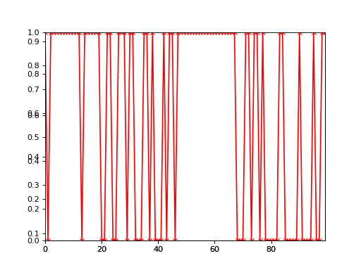
>>> bpplt.plot(Z)
>>> bpplt.plot(1-weather, color='r', marker='x')

(Source code, png, hires.png, pdf)

The black line shows the posterior probability of rain and the red line and crosses show the true state. Clearly, the method is not able to infer the weather very accurately in this case because the activies do not give that much information about the weather.

Unknown parameters

In this example, we consider unknown parameters for the Markov process and different emission distribution.

Data

We generate data from three 2-dimensional Gaussian distributions with different mean vectors and common standard deviation:

>>> import numpy as np
>>> mu = np.array([ [0,0], [3,4], [6,0] ])
>>> std = 2.0

Thus, the number of clusters is three:

>>> K = 3

And the number of samples is 200:

>>> N = 200

Each initial state is equally probable:

>>> p0 = np.ones(K) / K

State transition matrix is such that with probability 0.9 the process stays in the same state. The probability to move one of the other two states is 0.05 for both of those states.

>>> q = 0.9
>>> r = (1-q) / (K-1)
>>> P = q*np.identity(K) + r*(np.ones((3,3))-np.identity(3))

Simulate the data:

>>> y = np.zeros((N,2))
>>> z = np.zeros(N)
>>> state = np.random.choice(K, p=p0)
>>> for n in range(N):
...     z[n] = state
...     y[n,:] = std*np.random.randn(2) + mu[state]
...     state = np.random.choice(K, p=P[state])

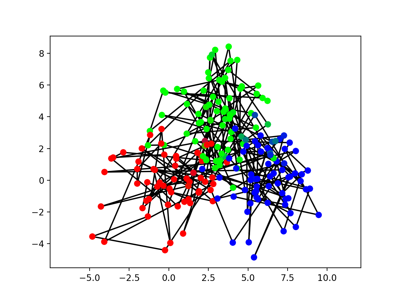
Then, let us visualize the data:

>>> bpplt.pyplot.figure()
<matplotlib.figure.Figure object at 0x...>
>>> bpplt.pyplot.axis('equal')
(...)
>>> colors = [ [[1,0,0], [0,1,0], [0,0,1]][int(state)] for state in z ]
>>> bpplt.pyplot.plot(y[:,0], y[:,1], 'k-', zorder=-10)
[<matplotlib.lines.Line2D object at 0x...>]
>>> bpplt.pyplot.scatter(y[:,0], y[:,1], c=colors, s=40)
<matplotlib.collections.PathCollection object at 0x...>

(Source code, png, hires.png, pdf)

Consecutive states are connected by a solid black line and the dot color shows the true class.

Model

Now, assume that we do not know the parameters of the process (initial state probability and state transition probabilities). We give these parameters quite non-informative priors, but it is possible to provide more informative priors if such information is available:

>>> from bayespy.nodes import Dirichlet
>>> a0 = Dirichlet(1e-3*np.ones(K))
>>> A = Dirichlet(1e-3*np.ones((K,K)))

The discrete Markov chain is constructed as:

>>> Z = CategoricalMarkovChain(a0, A, states=N)

Now, instead of using categorical emission distribution as before, we’ll use Gaussian distribution. For simplicity, we use the true parameters of the Gaussian distributions instead of giving priors and estimating them. The known standard deviation can be converted to a precision matrix as:

>>> Lambda = std**(-2) * np.identity(2)

Thus, the observed process is a Gaussian mixture with cluster assignments from the hidden Markov process Z:

>>> from bayespy.nodes import Gaussian
>>> Y = Mixture(Z, Gaussian, mu, Lambda)

Note that Lambda does not have cluster plate axis because it is shared between the clusters.

Inference

Let us use the simulated data:

>>> Y.observe(y)

Because VB takes all the random variables, we need to provide A and a0 also:

>>> Q = VB(Y, Z, A, a0)

Then, run VB iteration until convergence:

>>> Q.update(repeat=1000)
Iteration 1: loglike=-9.963054e+02 (... seconds)
...
Iteration 8: loglike=-9.235053e+02 (... seconds)
Converged at iteration 8.

Results

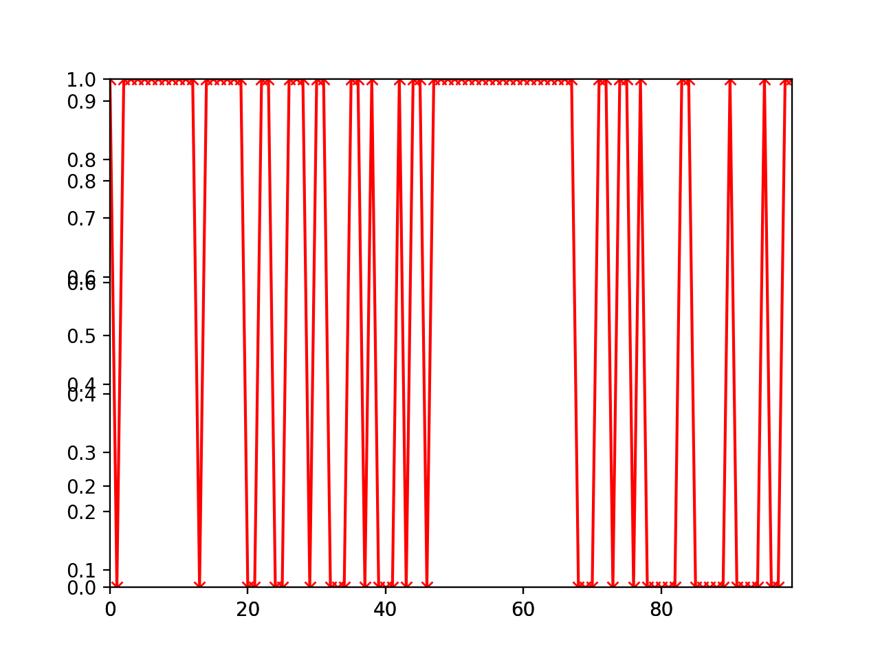
Plot the classification of the data similarly as the data:

>>> bpplt.pyplot.figure()
<matplotlib.figure.Figure object at 0x...>
>>> bpplt.pyplot.axis('equal')
(...)
>>> colors = Y.parents[0].get_moments()[0]
>>> bpplt.pyplot.plot(y[:,0], y[:,1], 'k-', zorder=-10)
[<matplotlib.lines.Line2D object at 0x...>]
>>> bpplt.pyplot.scatter(y[:,0], y[:,1], c=colors, s=40)
<matplotlib.collections.PathCollection object at 0x...>

(Source code, png, hires.png, pdf)

The data has been classified quite correctly. Even samples that are more in the region of another cluster are classified correctly if the previous and next sample provide enough evidence for the correct class. We can also plot the state transition matrix:

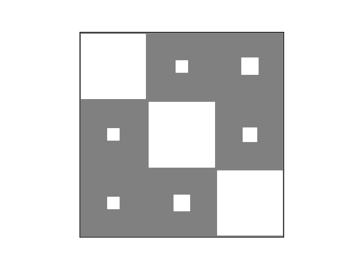
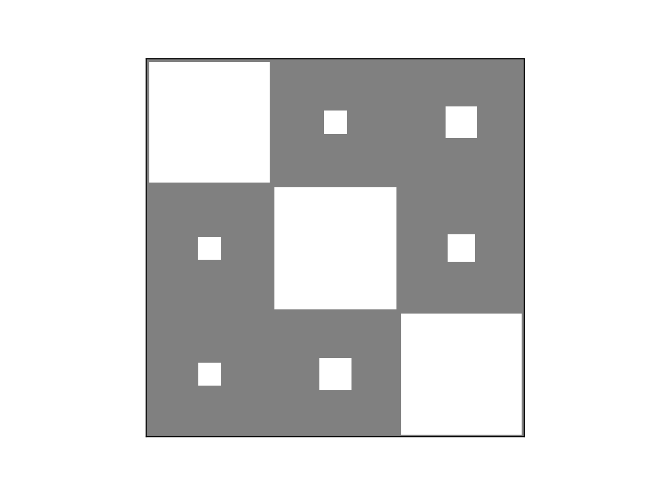
>>> bpplt.hinton(A)

(Source code, png, hires.png, pdf)

Clearly, the learned state transition matrix is close to the true matrix. The models described above could also be used for classification by providing the known class assignments as observed data to Z and the unknown class assignments as missing data.